Paths
A first introduction to paths was given in the
tutorial. In this guide we'll explore some of the more powerful operations that can be performed on paths.
Before discussing path sliders in the next section, we must introduce the concepts of spline time and arc time. Recall that a path is a sequence of connected cubic splines, and that each spline segment can be parameterized by a scalar in the range 0 to 1.
First, a spline time is a real number used to refer to points on paths. The integer part refers to a spline segment, with zero being the first segment, while the fractional part refers to a point on that segment. Second, an arc time is a length used to refer to points on paths. The length is simply the arc length from the beginning of the path to the point being referred to.
Note that spline time makes no sense from a geometric point of view. To see this, note that any spline segment can be divided into several shorter spline segments, and that while this does not change the geometry of the path, it changes the interpretation of spline times along the path. On the other hand, spline time is very natural from a computer representation point of view. Therefore, all arc times are converted to spline times internally in Shapes, a procedure which relies on numeric integration.
While the numeric integration required to work with arc time may seem costly from a computational point of view, it is believed that working with features of geometry rather then representation is such an important tool that it is worth while the extra computation time. While this argument may not have been feasible in the times when MetaPost was designed, the computational power of personal computers has increased by huge amounts since then, and we think that computing arc lengths is a good use of this power. Hence, users are recommended to avoid thinking in terms of spline time unless working explicitly with the underlying path representation.
A path slider, generally referred to as just slider, is a location on a particular path. It is the natural result of any operation that selects a point on a path, and gives access to local characteristics of the path such as tangent its direction and curvature. In Shapes, a sub-range of a path is constructed by connecting one slider at the beginning of the range with another slider at the end of the range.
There are two types of sliders, depending on whether their paths are contained in 2
d or 3
d, see
§PathSlider and
§PathSlider3D, for details.
As the name suggests, a slider can be used to move along the path. By adding
§Float or
§Length values to a slider, one obtains a new slider at the given distance from the original slider;
§Float values move in terms of spline time, while
§Length values move in terms of arc length.
The simplest operations that yield sliders on a path are either to access the fields
begin or
end, or to
apply the path like a function to a
§Float value to construct a slider with the given spline time. Similarly, if the path is applied to a
§Length value, one obtains a slider at the given arc time.
The function
..Shapes..Layout..mspoint (read it as
mediation-slide point) is a convenient way to specify the arc time relative to the arc length of the path itself.
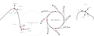
The most often used field of a slider is its location in space. The name of this field is p. This along with other fields and slider use is shown in the next example. Note that there are additional fields in 3d, and that it is not obvious how to best extend the definitions from 2d to 3d.
| Sliders |
|---|
 |
|
Sliders. Given a slider, other sliders can be specified relative to the first one, either in terms of distance or in terms of spline time. Then, there are many fields to access to get both geometric and representation-related information about the particular point along the path. The right part of the picture shows that the velocity field v varies along a circle, so this is an example of a non-geometric field.
Note that arrows indicating direction have been given an arbitrary length.
|
|
| Source:
show/hide
—
visit
|
##needs ..Applications..Blockdraw

##preamble \usepackage[squaren]{SIunits}

##lookin ..Shapes
##lookin ..Shapes..Geometry
##lookin ..Applications..Blockdraw

pathStyle: Traits..@width: 1bp
labelStyle: Traits..@width: 0.3bp & Traits..@stroking:[Traits..gray 0.5] & Traits..@dash:[Traits..dashpattern 1mm 1mm]
labelHead: [Graphics..ShapesArrow width:2mm ...]
onPathMark: Traits..@nonstroking:Traits..RGB..RED | [Graphics..fill [Geometry..circle 1mm]]
dirStyle: Traits..@width: 0.7bp
dirHead: [Graphics..ShapesArrow width:2mm ...]
dirLen: 1cm
sourceFont: Text..@size:9bp & Text..@font:Text..Font..COURIER

path: Geometry..@defaultunit:1%C | (0cm,0cm)--(2cm,2cm)>(^)--(^)<(5cm,~2cm)>(^)--(^)<(7cm,~2cm)

IO..•page << pathStyle | [Graphics..stroke path]

/**
 ** Here, the slider s0 "slides" by distance and arctime to yield the sliders s1 and s2.
 **/
s0: [Debug..locate [path 1.2]]
s1: [Debug..locate s0+4.7cm]
s2: [Debug..locate s0+1]

IO..•stdout << `s0: ´ << [String..sprintf `spline time: %.3g´ s0.time] << `, ´ << [String..sprintf `arc time: %.3gcm´ s0.length/1cm] << "{n}
IO..•stdout << `s1: ´ << [String..sprintf `spline time: %.3g´ s1.time] << `, ´ << [String..sprintf `arc time: %.3gcm´ s1.length/1cm] << "{n}
IO..•stdout << `s2: ´ << [String..sprintf `spline time: %.3g´ s2.time] << `, ´ << [String..sprintf `arc time: %.3gcm´ s2.length/1cm] << "{n}

/**
 ** Annotate s0
 **/
{
  /**
   ** Mark the point where the slider sits, and label it.
   **/
  IO..•page << [shift s0.p] [] onPathMark
  lblPoint: s0.p+(1cm,0.5cm)
  IO..•page << [putlabelRight sourceFont | ( Text..newText << `s0.p´ ) lblPoint ~1]
  IO..•page << labelStyle | [Graphics..stroke lblPoint--s0.p head:labelHead]

  /**
   ** Show the tangent direction, <T>.
   **/
  Tend: s0.p + dirLen*s0.T
  IO..•page << dirStyle | [Graphics..stroke s0.p--Tend head:dirHead]
  IO..•page << [putlabelRight sourceFont | ( Text..newText << `s0.T´ ) Tend 0]

  /**
   ** Show the normal direction, <N>.  Note that it does not depend on curvature, but is always counter-clockwise from the tangent.
   **/
  Nend: s0.p + dirLen*s0.N
  IO..•page << dirStyle | [Graphics..stroke s0.p--Nend head:dirHead]
  IO..•page << [putlabelAbove sourceFont | ( Text..newText << `s0.N´ ) Nend 0]

  /**
   ** To show the inverse curvature, <ik>, we draw a circle with this radius, centered in the normal direction.
   ** Note that the sign of <ik> is defined such that the center of the circle is shifted <N> * <ik> from <p>,
   ** even though the direction of the normal s0.N does not depend on curvature (as it sometomes does in mathematics).
   **/
  center: s0.p + s0.N * s0.ik
  IO..•page << labelStyle | [Graphics..stroke [shift center] [] [Geometry..circle s0.ik]]
        << labelStyle | [Graphics..stroke s0.p--center head:labelHead]
        << [putlabelBelow sourceFont | ( Text..newText << `s0.N * s0.ik´ ) center 0]
}

/**
 ** Annotate s1
 **/
{
  IO..•page << [shift s1.p] [] onPathMark
  lblPoint: s1.p+(~1cm,0.5cm)
  IO..•page << [putlabelLeft sourceFont | ( Text..newText << `s1.p´ ) lblPoint ~1]
  IO..•page << labelStyle | [Graphics..stroke lblPoint--s1.p head:labelHead]

  Tend: s1.p + dirLen*s1.T
  IO..•page << dirStyle | [Graphics..stroke s1.p--Tend head:dirHead]
  IO..•page << [putlabelBelow sourceFont | ( Text..newText << `s1.T´ ) Tend 0]

  Nend: s1.p + dirLen*s1.N
  IO..•page << dirStyle | [Graphics..stroke s1.p--Nend head:dirHead]
  IO..•page << [putlabelAbove sourceFont | ( Text..newText << `s1.N´ ) Nend 1]

  center: s1.p + s1.N * s1.ik
  IO..•page << labelStyle | [Graphics..stroke [shift center] [] [Geometry..circle s1.ik]]
        << labelStyle | [Graphics..stroke s1.p--center head:labelHead]
        << [putlabelAbove sourceFont | ( Text..newText << `s1.N * s1.ik´ ) center 0]
}

/**
 ** Annotate s2
 **/
{
  IO..•page << [shift s2.p] [] onPathMark
  lblPoint: s2.p+(1cm,~0.5cm)
  IO..•page << [putlabelRight sourceFont | ( Text..newText << `s2.p´ ) lblPoint ~1]
  IO..•page << labelStyle | [Graphics..stroke lblPoint--s2.p head:labelHead]
}


/**
 ** We now illustrate that the veolcity is not a geometric property, since it is not constant along a circle.
 ** This also illustrates how the field <looped> can be used to traverse closed paths.  The field <past> serves
 ** a similar purpose for open paths.
 **/
{
  c: (13cm,0)
  circ: [shift c] [] [Geometry..circle 2cm]
  IO..•page << pathStyle | [Graphics..stroke circ]
        << [[Data..range '0 '3].foldl \ p e → ( p & [[shift [circ e*1].p] onPathMark] ) Graphics..null]
  upAngle: \ d →
  {
    a: [angle d]
    [if ~90° ≤ a and a ≤ 90°
      a
      a + 180°]
  }
  helper: \ sl →
    [if (not sl.looped)
      {
        pth: sl.p--(sl.p+sl.T*sl.v)
        slMid: (pth.end - 1cm)
        [Graphics..stroke pth head:dirHead]
        &
        [[shift pth.begin.p] [Graphics..stroke pth.begin.N*2bp--pth.begin.N*~2bp]]
        &
[[shift slMid.p+1mm*[dir [upAngle slMid.T]+90°]]*[rotate [upAngle slMid.T]] [Layout..center [Graphics..TeX [String..sprintf `$\unit{%.3g}{\centi\metre}$´ sl.v/1cm]] (0,~1)]]
        &
        [helper sl+1.6cm]
      }
      Graphics..null]
  IO..•page << dirStyle | [helper circ.begin]
  IO..•page << [shift c] [] [Layout..center [Graphics..TeX `The velocity $v$´] (0,0)]

  /** While we are working with a closed path, we also illustrate the <mod> field.  It is a slider at the same location, but with a spline time in the range
   ** zero to the duration of the path.
   **/
  sLoop: [circ 5.5]
  sMod: sLoop.mod
  IO..•stdout << `sLoop: ´ << [String..sprintf `spline time: %.3g´ sLoop.time] << `, ´ << [String..sprintf `arc time: %.3gcm´ sLoop.length/1cm] << "{n}
  IO..•stdout << `sMod: ´ << [String..sprintf `spline time: %.3g´ sMod.time] << `, ´ << [String..sprintf `arc time: %.3gcm´ sMod.length/1cm] << "{n}
}

/**
 ** Finally, we show very briefly the difference between normal and reverse fields by comparing <T> and <rT> at a corner.
 **/
{
  pth: Geometry..@defaultunit:1%C | [[shift (18cm,0)] (0cm,0cm)>(^90°)--(2cm^170°)<(2cm,2cm)>(2cm^~45°)--(^90°)<(4cm,0cm)]
  IO..•page << pathStyle | [Graphics..stroke pth]
  s: [pth 1]

  IO..•page << [shift s.p] [] onPathMark
  lblPoint: s.p+(0cm,1.5cm)
  IO..•page << [putlabelAbove sourceFont | ( Text..newText << `s.p´ ) lblPoint 0]
  IO..•page << labelStyle | [Graphics..stroke lblPoint--s.p head:labelHead]

  {
    /** First the forward versions of tangent and normal.
     **/
  Tend: s.p + dirLen*s.T
  IO..•page << dirStyle | [Graphics..stroke s.p--Tend head:dirHead]
  IO..•page << [putlabelBelow sourceFont | ( Text..newText << `s.T´ ) Tend 0]

  Nend: s.p + dirLen*s.N
  IO..•page << dirStyle | [Graphics..stroke s.p--Nend head:dirHead]
  IO..•page << [putlabelAbove sourceFont | ( Text..newText << `s.N´ ) Nend ~1]
  }

  {
    /** Then the reverse versions.
     **/
  Tend: s.p + dirLen*s.rT
  IO..•page << dirStyle | [Graphics..stroke s.p--Tend head:dirHead]
  IO..•page << [putlabelAbove sourceFont | ( Text..newText << `s.rT´ ) Tend 1]

  Nend: s.p + dirLen*s.rN
  IO..•page << dirStyle | [Graphics..stroke s.p--Nend head:dirHead]
  IO..•page << [putlabelBelow sourceFont | ( Text..newText << `s.rN´ ) Nend 1]
  }

}
|
|
| stdout:
show/hide
|
s0: spline time: 1.2, arc time: 4.33cm
s1: spline time: 1.88, arc time: 9.03cm
s2: spline time: 2.2, arc time: 9.95cm
sLoop: spline time: 5.5, arc time: 17.3cm
sMod: spline time: 1.5, arc time: 4.72cm
|
In this section, we shall describe the powerful ways of referring to points (one at a time) on paths. Although most of these methods are defined and implemented in terms of optimization and that this may seem expensive from a computational point of view, one should keep in mind that precise computation of curve lengths (arc times) can be rather expensive too. Hence, try to use the powerful abstractions presented here whenever you think they are the best match for your thinking, and resort only to less expensive alternatives when too lengthy computations are a fact.
As usual, we concentrate on the methods in 2d, and make at most minor comments regarding the 3d counterparts.
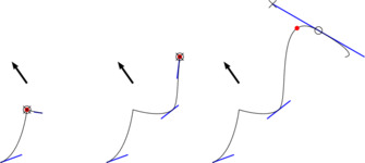
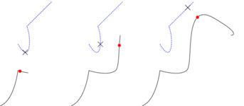
Let us begin with a concept which appears also in MetaPost, namely to find the first point on a path where the path has a certain direction. In one does not specify the direction, but maximize the function in an orthogonal direction. This avoids undefined results when the given direction is never attained, and generalizes immediately to 3
d. The function that does the job is
..Shapes..Geometry..maximizer. Sometimes, one is only interested in a coarse maximization, looking only at the points where the path goes through a path point, in which case
..Shapes..Geometry..pathpoint_maximizer does the job. A third option is to maximize over all the control points of the path (the convex hull of which is known to contain the path). Note, though, that while
..Shapes..Geometry..maximizer and
..Shapes..Geometry..pathpoint_maximizer yield a
§PathSlider,
..Shapes..Geometry..controlling_maximizer cannot do this but returns a
§Coords since the maximizing point is not on the path in general.
| Maximizers |
|---|
 |
|
Maximizing in the direction indicated by the arrow. Control points of the path are marked by connecting them with blue lines to the path point they belong to. The first maximizing point on the path is marked with a red spot, the first maximizing point through a path point is marked with a small circle, and the maximizing point among all the control points is marked with a cross.
|
|
| Source:
show/hide
—
visit
|
##lookin ..Shapes
##lookin ..Shapes..Geometry

n: [dir 125°]

pth: Geometry..@defaultunit:1%C | (0cm,0cm)>(^20°)--(1cm,2cm)--(^)<(2.5cm,2cm)>(^)--(2cm^)<(4cm,5cm)>(^~30°)--(^)<(5cm,4cm)

circMark: Traits..@width:0.5bp | [Graphics..stroke [Geometry..circle 4bp]]
crossMark: Traits..@width:0.5bp | [Graphics..stroke (~4bp,~4bp)--(4bp,4bp) & (~4bp,4bp)--(4bp,~4bp)]

helper: \ pth →
{
  ( Traits..@width:2bp | [Graphics..stroke (1cm,3cm)--(+n*1cm) head:Graphics..ShapesArrow] )
  &
  ( Traits..@width:1bp & Traits..@stroking:Traits..RGB..BLUE | [Graphics..stroke [Geometry..controlling pth]] )
  &
  ( Traits..@width:0.5bp | [Graphics..stroke pth] )
  &
  ( Traits..@width:5bp & Traits..@stroking:Traits..RGB..RED | [Graphics..spot [Geometry..maximizer pth n].p] )
  &
  ( [shift [Geometry..pathpoint_maximizer pth n].p] [] circMark )
  &
  ( [shift [Geometry..controlling_maximizer pth n]] [] crossMark )
}

IO..•page << [helper pth.begin--[pth 1.5]]
      << [shift (4cm,0cm)] [] [helper pth.begin--[pth 2.5]]
      << [shift (8cm,0cm)] [] [helper pth]
|
| Point approximators |
|---|
 |
|
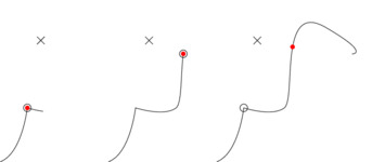
Minimizing the distance to the point marked with a cross. The first maximizing point on the path is marked with a red spot, and the first maximizing point through a path point is marked with a small circle.
|
|
| Source:
show/hide
—
visit
|
##lookin ..Shapes
##lookin ..Shapes..Geometry

a: (1.5cm,4.5cm)

pth: Geometry..@defaultunit:1%C | (0cm,0cm)>(^20°)--(1cm,2cm)--(^)<(2.5cm,2cm)>(^)--(2cm^)<(4cm,5cm)>(^~30°)--(^)<(5cm,4cm)

circMark: Traits..@width:0.5bp | [Graphics..stroke [Geometry..circle 4bp]]
crossMark: Traits..@width:0.5bp | [Graphics..stroke (~4bp,~4bp)--(4bp,4bp) & (~4bp,4bp)--(4bp,~4bp)]

helper: \ pth →
{
  [[shift a] crossMark]
  &
  ( Traits..@width:0.5bp | [Graphics..stroke pth] )
  &
  ( Traits..@width:5bp & Traits..@stroking:Traits..RGB..RED | [Graphics..spot [Geometry..approximator pth a].p] )
  &
  ( [shift [Geometry..pathpoint_approximator pth a].p] [] circMark )
}

IO..•page << [helper pth.begin--[pth 1.5]]
      << [shift (4cm,0cm)] [] [helper pth.begin--[pth 2.5]]
      << [shift (8cm,0cm)] [] [helper pth]
|
Another concept for point references is that of intersection points. This has only been implemented in 2
d as the function
..Shapes..Geometry..intersection (where the intersection with another path can be found), since Shapes does not support the abstraction of a general surface in 3
d. Note that there may be no intersection at all, in which case
..Shapes..Geometry..intersection will invoke an error handler, see the following example.
| Path intersection |
|---|
 |
|
Finding the first point on the solid black path (direction indicated by the arrow) where it intersects with the dashed blue path (direction not important). The intersection is marked with a red spot, and an error handler is used to treat the case when there is no intersection.
|
|
| Source:
show/hide
—
visit
|
##lookin ..Shapes
##lookin ..Shapes..Geometry

a: (1.5cm,4.5cm)

pth: Geometry..@defaultunit:1%C | (0cm,0cm)>(^20°)--(1cm,2cm)--(^)<(2.5cm,2cm)>(^)--(2cm^)<(4cm,5cm)>(^~30°)--(^)<(5cm,4cm)

circMark: Traits..@width:0.5bp | [Graphics..stroke [circle 4bp]]
crossMark: Traits..@width:0.5bp | [Graphics..stroke (~4bp,~4bp)--(4bp,4bp) & (~4bp,4bp)--(4bp,~4bp)]

helper: \ pth2 →
{
  ( Traits..@width:0.5bp & Traits..@stroking:Traits..RGB..BLUE & Traits..@dash:[Traits..dashpattern 2bp 1bp] | [Graphics..stroke pth2] )
  &
  ( Traits..@width:0.5bp | [Graphics..stroke pth] )
  &
  ( Traits..@width:0.0bp | [Graphics..stroke [pth 0.5cm]--[pth 1cm] head:[Graphics..ShapesArrow width:2mm ...]] )
  &
  (escape_continuation cont
  /** The two options for @handler_NoIntersection below deal with the situation in quite different ways.
   ** The first uses an escape continuation to replace the usual spot with nothing (null).
   ** The second makes the intersection return the beginning of the path, although there is no intersection there.
   **/
      @handler_NoIntersection: ( \ pth1 pth2 → (escape_continue cont Graphics..null) )
|**      @handler_NoIntersection: ( \ pth1 pth2 → pth.begin )
    & Traits..@width:5bp
    & Traits..@stroking:Traits..RGB..RED
    | [Graphics..spot [intersection pth pth2].p] )
}

IO..•page << [helper [shift (1.3cm,4cm)][][circle 0.5cm]]
      << [shift (6cm,0cm)] [] [helper [shift (1cm,2.5cm)][][circle 1.5cm]]
      << [shift (12cm,0cm)] [] [helper [shift (2cm,2cm)][][circle 3cm]]
|
Finally, there is a generalization of intersection of paths which generalizes to 3
d, and that is to find the point where the path is closest to the other path. Again,
..Shapes..Geometry..approximator is the interface — depending on argument types, it will dispatch to the appropriate path-to-point or path-to-path algorithm. Note that, in the absence of intersections, it is ill-conditioned to speak of order between equally closed points (since the distance cannot be computed exactly anyway). The first example shows basic use, the following example shows how
..Shapes..Geometry..approximator is used as an alternative to
..Shapes..Geometry..intersection.
| Path approximator |
|---|
 |
|
Minimizing the distance to the dashed blue path. The closest point on the path is marked with a red spot. The corresponding point on the target path is found using path-to-point approximation, which is significantly cheaper, although it could be argued that this point should also be returned somehow from the path-to-path approximation.
|
|
| Source:
show/hide
—
visit
|
##lookin ..Shapes
##lookin ..Shapes..Geometry

pth2: Geometry..@defaultunit:1%C | (1cm,3.5cm)>(^~60°)--(^~60°)<(1.5cm,4.5cm)--(+(2cm*[dir 45°]))

pth: Geometry..@defaultunit:1%C | (0cm,0cm)>(^20°)--(1cm,2cm)--(^)<(2.5cm,2cm)>(^)--(2cm^)<(4cm,5cm)>(^~30°)--(^)<(5cm,4cm)

crossMark: Traits..@width:0.5bp | [Graphics..stroke (~4bp,~4bp)--(4bp,4bp) & (~4bp,4bp)--(4bp,~4bp)]

helper: \ pth →
{
  sl: [Geometry..approximator pth pth2]
  ( Traits..@width:0.5bp & Traits..@stroking:Traits..RGB..BLUE & Traits..@dash:[Traits..dashpattern 2bp 1bp] | [Graphics..stroke pth2] )
  &
  ( Traits..@width:0.5bp | [Graphics..stroke pth] )
  &
  ( Traits..@width:5bp & Traits..@stroking:Traits..RGB..RED | [Graphics..spot sl.p] )
  &
  [[shift sl.info.other.p] crossMark]
}

IO..•page << [helper pth.begin--[pth 1.5]]
      << [shift (4cm,0cm)] [] [helper pth.begin--[pth 2.5]]
      << [shift (8cm,0cm)] [] [helper pth]
|
| Path intersection by approximation |
|---|
 |
|
|
|
| Source:
show/hide
—
visit
|
##lookin ..Shapes
##lookin ..Shapes..Geometry

a: (1.5cm,4.5cm)

pth: Geometry..@defaultunit:1%C | (0cm,0cm)>(^20°)--(1cm,2cm)--(^)<(2.5cm,2cm)>(^)--(2cm^)<(4cm,5cm)>(^~30°)--(^)<(5cm,4cm)

circMark: Traits..@width:0.5bp | [Graphics..stroke [Geometry..circle 4bp]]
crossMark: Traits..@width:0.5bp | [Graphics..stroke (~4bp,~4bp)--(4bp,4bp) & (~4bp,4bp)--(4bp,~4bp)]

helper: \ pth2 →
{
  ( Traits..@width:0.5bp & Traits..@stroking:Traits..RGB..BLUE & Traits..@dash:[Traits..dashpattern 2bp 1bp] | [Graphics..stroke pth2] )
  &
  ( Traits..@width:0.5bp | [Graphics..stroke pth] )
  &
  ( Traits..@width:0.0bp | [Graphics..stroke [pth 0.5cm]--[pth 1cm] head:[Graphics..ShapesArrow width:2mm ...]] )
  &
  ( Traits..@width:5bp & Traits..@stroking:Traits..RGB..RED | [Graphics..spot [Geometry..approximator pth pth2].p] )
}

IO..•page << [helper [shift (1.3cm,4cm)][][Geometry..circle 0.5cm]]
      << [shift (6cm,0cm)] [] [helper [shift (1cm,2.5cm)][][Geometry..circle 1.5cm]]
      << [shift (12cm,0cm)] [] [helper [shift (2cm,2cm)][][Geometry..circle 3cm]]
|
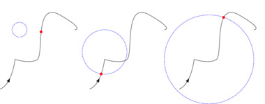
OK, that's pretty much all for now; more point references may be added in the future. However, it should be mentioned here that there is no built in support for evaluating the point references on anything smaller than the whole path. The last example in this section shows how this can be done manually.
| Subpath intersection |
|---|
 |
|
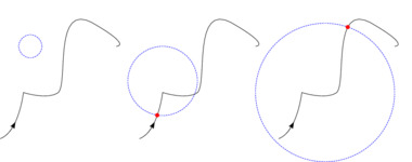
Finding the first point on the solid black path (direction indicated by the arrow), between the two circles, where it intersects with the dashed blue path (direction not important). The intersection is marked with a red spot. Note that one must make use of arc length rather than spline time to relate the slider on the sub path to a slider on the whole path (which makes this a bit more expensive and inaccurate compared to what a built-in solution could offer).
|
|
| Source:
show/hide
—
visit
|
##lookin ..Shapes
##lookin ..Shapes..Geometry

a: (1.5cm,4.5cm)

pth: Geometry..@defaultunit:1%C | (0cm,0cm)>(^20°)--(1cm,2cm)--(^)<(2.5cm,2cm)>(^)--(2cm^)<(4cm,5cm)>(^~30°)--(^)<(5cm,4cm)
sl1: [pth 2cm]
sl2: [pth 4cm]

circMark: Traits..@width:0.5bp | [Graphics..stroke [Geometry..circle 4bp]]
crossMark: Traits..@width:0.5bp | [Graphics..stroke (~4bp,~4bp)--(4bp,4bp) & (~4bp,4bp)--(4bp,~4bp)]

subpath_intersection: \ sl1 sl2 pth → (sl1+[Geometry..intersection sl1--sl2 pth].length)

helper: \ pth2 →
{
  ( Traits..@width:0.5bp & Traits..@stroking:Traits..RGB..BLUE & Traits..@dash:[Traits..dashpattern 2bp 1bp] | [Graphics..stroke pth2] )
  &
  ( Traits..@width:0.5bp | [Graphics..stroke pth] )
  &
  ( Traits..@width:0.0bp | [Graphics..stroke [pth 0.5cm]--[pth 1cm] head:[Graphics..ShapesArrow width:2mm ...]] )
  &
  [[shift sl1.p] circMark]
  &
  [[shift sl2.p] circMark]
  &
  ( Traits..@width:5bp & Traits..@stroking:Traits..RGB..RED | [Graphics..spot [subpath_intersection sl1 sl2 pth2].p] ) /** We know that there will be an intersection, so no error handler this time. **/
}

IO..•page << [helper (0cm,0.3cm)--(5cm,5cm)]
|
There are operations on paths that despite a seemingly simple abstraction turn out very complicated to implement to a reasonable degree of accuracy. The design choice of Shapes was not to provide lousy implementations of these abstractions, but to provide simpler operations that can be implemented accurately and that will allow users to make their own approximations of the difficult abstractions. Basically, this comes down to means for folding over the discrete spline points defining a path, and means for generating a sufficiently dense sampling of the path. Currently, there are only means for upsampling, that is, to generate a representation that uses more points to define the same geometric path. The opposite, downsampling may be added in the future, but right now it is not even clear how the operation should be defined abstractly (note that downsampling will require the original path to be approximated somehow).
In this section, we shall discuss the available methods for upsampling. One of the methods refers to the Bezier spline representation of the new path, while the other methods have geometric meanings.
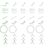
Beginning with the method which is not geometric, we have
..Shapes..Geometry..upsample_balance, which will divide each spline in two, such that the velocity is continuous through the new sample point. This will imply that the the two interpolation points around the new sample point are at equal distance (and opposite), hence the
balance part of the name. It turns out that the sample point will be at spline time 0.5, so the operation is very cheap. Use this method if you need speed more than good properties of the upsampled path.
The method
..Shapes..Geometry..upsample_inflections adds samples where there were inflections on the spline segments of the original path. The new path will only have spline segments without inflections, which can be a useful thing when reasoning about the path in terms of its spline segment representation.
The method
..Shapes..Geometry..upsample_bends may be the most useful method of them all. It begins sampling at inflections (see
..Shapes..Geometry..upsample_inflections), and then it makes sure that each spline segment bends at most some given angle. Since it is often the parts of a path where it bends most that are difficult to work with, this method often gives you samples where you need them most.
The example below show the various methods applied to a variety of paths.
| Upsampling |
|---|
 |
|
Various ways of upsampling a path.
|
|
| Source:
show/hide
—
visit
|
##lookin ..Shapes
##lookin ..Shapes..Geometry

pathpoints:
{
  helper: \ sl → [if sl.looped Data..nil [Data..cons sl [helper sl+1]]]
  \ pth → [helper pth.begin]
}


sstroke: \ pth →
( (Traits..@stroking:Traits..RGB..RED & Traits..@width:(0.5*Traits..@width) | [[pathpoints pth].foldl \ p sl → ( p & [Graphics..stroke [shift sl.p][]( (sl.N*3*Traits..@width)--(sl.N*~3*Traits..@width) )] )  Graphics..null])
   &
   [Graphics..stroke pth]
)

cstroke: \ pth →
(
  (Traits..@stroking:Traits..RGB..GREEN & Traits..@width:(2*Traits..@width) | [Graphics..stroke [Geometry..controlling pth]] )
  &
  (Traits..@stroking:Traits..RGB..RED & Traits..@width:(0.5*Traits..@width) | [[pathpoints pth].foldl \ p sl → ( p & [Graphics..stroke [shift sl.p][]( (sl.N*3*Traits..@width)--(sl.N*~3*Traits..@width) )] )  Graphics..null])
  &
  [Graphics..stroke pth]
)

{
  pth: (~2cm,0cm)<(0cm,0cm)>(2cm,~1cm)--(1cm,3cm)<(2cm,1cm)>(3cm,1cm)
  IO..•page << [sstroke pth]
  IO..•page << [cstroke [upsample_balance [shift (~5cm,0)][]pth]]
  IO..•page << [sstroke [upsample_inflections [shift (5cm,0)][]pth]]
  IO..•page << [sstroke [upsample_bends 60° [shift (10cm,0)][]pth]]
  IO..•page << [sstroke [upsample_every 1cm [shift (15cm,0)][]pth]]
}

{
  pth: [[shift (0,~2cm)] (0cm,0cm)>(~2cm,0.2cm)--(3cm,~0.2cm)<(2cm,0cm)]
  IO..•page << [sstroke pth]
  IO..•page << [cstroke [upsample_balance [shift (~5cm,0)][]pth]]
  IO..•page << [sstroke [upsample_inflections [shift (5cm,0cm)][]pth]]
  IO..•page << [sstroke [upsample_bends 60° [shift (10cm,0)][]pth]]
  IO..•page << [sstroke [upsample_every 1cm [shift (15cm,0)][]pth]]
}
{
  pth: [[shift (0,~3cm)] (0cm,0cm)>(~2cm,0.2cm)--(3cm,0.2cm)<(2cm,0.1cm)]
  IO..•page << [sstroke pth]
  IO..•page << [cstroke [upsample_balance [shift (~5cm,0)][]pth]]
  IO..•page << [sstroke [upsample_inflections [shift (5cm,0cm)][]pth]]
  IO..•page << [sstroke [upsample_bends 60° [shift (10cm,0)][]pth]]
  IO..•page << [sstroke [upsample_every 1cm [shift (15cm,0)][]pth]]
}
{
  pth: [[shift (0,~4cm)] (0cm,0cm)>(~2cm,0cm)--(3cm,0cm)<(2cm,0cm)]
  IO..•page << [sstroke pth]
  IO..•page << [cstroke [upsample_balance [shift (~5cm,0)][]pth]]
  IO..•page << [sstroke [upsample_inflections [shift (5cm,0cm)][]pth]]
  IO..•page << [sstroke [upsample_bends 60° [shift (10cm,0)][]pth]]
  IO..•page << [sstroke [upsample_every 1cm [shift (15cm,0)][]pth]]
}

{
  pth: [[shift (0,~7cm)] (~1cm,~0.5cm)--(2cm,1cm)]
  IO..•page << [sstroke pth]
  IO..•page << [cstroke [upsample_balance [shift (~5cm,0)][]pth]]
  IO..•page << [sstroke [upsample_inflections [shift (5cm,0cm)][]pth]]
  IO..•page << [sstroke [upsample_bends 60° [shift (10cm,0)][]pth]]
  IO..•page << [sstroke [upsample_every 1cm [shift (15cm,0)][]pth]]
}

{
  pth: [[shift (0,~10cm)] (~2cm,0cm)<(0cm,0cm)>(2cm,~1cm)--(1cm,3cm)<(2cm,1cm)>(3cm,1cm)--cycle]
  IO..•page << [sstroke pth]
  IO..•page << [cstroke [upsample_balance [shift (~5cm,0)][]pth]]
  IO..•page << [sstroke [upsample_inflections [shift (5cm,0)][]pth]]
  IO..•page << [sstroke [upsample_bends 60° [shift (10cm,0)][]pth]]
  IO..•page << [sstroke [upsample_every 1cm [shift (15cm,0)][]pth]]
}

{
  pth: [[shift (0,~13cm)] [circle 2cm]]
  IO..•page << [sstroke pth]
  IO..•page << [cstroke [upsample_balance [shift (~5cm,0)][]pth]]
  IO..•page << [sstroke [upsample_bends 40° [shift (10cm,0)][]pth]]
  IO..•page << [sstroke [upsample_every 1cm [shift (15cm,0)][]pth]]
}

{
  pth: [[shift (0,~17cm)] (0cm,0cm)>(2.5cm^45°)--(2.5cm^135°)<(2cm,0cm)]
  IO..•page << [sstroke pth]
  IO..•page << [cstroke [upsample_balance [shift (~5cm,0)][]pth]]
  IO..•page << [sstroke [upsample_inflections [shift (5cm,0cm)][]pth]]
  IO..•page << [sstroke [upsample_bends 60° [shift (10cm,0)][]pth]]
  IO..•page << [sstroke [upsample_every 1cm [shift (15cm,0)][]pth]]
}
{
  pth: [[shift (0,~19cm)] (0cm,0cm)>(2cm,2cm)--(0cm,2cm)<(2cm,0cm)]
  IO..•page << [sstroke pth]
  IO..•page << [cstroke [upsample_balance [shift (~5cm,0)][]pth]]
  IO..•page << [sstroke [upsample_inflections [shift (5cm,0cm)][]pth]]
  IO..•page << [sstroke [upsample_bends 60° [shift (10cm,0)][]pth]]
  IO..•page << [sstroke [upsample_every 1cm [shift (15cm,0)][]pth]]
}
{
  pth: [[shift (0,~21cm)] (0cm,0cm)>(4cm^45°)--(4cm^135°)<(2cm,0cm)]
  IO..•page << [sstroke pth]
  IO..•page << [cstroke [upsample_balance [shift (~5cm,0)][]pth]]
  IO..•page << [sstroke [upsample_inflections [shift (5cm,0cm)][]pth]]
  IO..•page << [sstroke [upsample_bends 60° [shift (10cm,0)][]pth]]
  IO..•page << [sstroke [upsample_every 1cm [shift (15cm,0)][]pth]]
}
|
We end this section with an example showing an application of upsampling. The seemingly simple abstraction is to compute a path, following a given path at a certain distance. Basically, one would like to be able to compute one of the boundaries of a stroke along the path, but it is easy to also imagine more interesting generalizations. The idea is easy as long as the path has a radius of curvature being larger than the distance between the original and the new path, but when it is not the situation gets much more involved, and it is for this reason the (very important) operation is not included in the kernel.
| Sidepaths |
|---|
 |
Application of upsampling: Computing side paths. Note that much of the interesting source code for this example is located in the extension ..Shapes..Geometry / pathmapping. |
|
| Source:
show/hide
—
visit
|
##needs ..Shapes..Geometry / pathmapping

##lookin ..Shapes
##lookin ..Shapes..Geometry

pathpoints:
{
  helper: \ sl → [if sl.looped Data..nil [Data..cons sl [helper sl+1]]]
  \ pth → [helper pth.begin]
}


sstroke: \ pth →
( (Traits..@stroking:Traits..RGB..BLACK | [[pathpoints pth].foldl \ p sl → ( p & [Graphics..stroke [shift sl.p][]( (sl.N*6*Traits..@width)--(sl.N*~5*Traits..@width) )] )  Graphics..null])
   &
   [Graphics..stroke pth]
)

cstroke: \ pth →
(
  (Traits..@stroking:Traits..RGB..GREEN & Traits..@width:(2*Traits..@width) | [Graphics..stroke [Geometry..controlling pth]] )
  &
  [sstroke pth]
)

testPth: Geometry..@defaultunit:1%C | (0cm,0cm)>(^~30°)--(^)<(2cm,3cm)>(^45°)--(^)<(5cm,2cm)>(^0°)--(6cm,2cm)--(8cm,4cm)

test: \ •dst pth method →
(
Traits..@width: 0.5bp
|
{
  •dst << Traits..@stroking:Traits..RGB..RED | [cstroke pth]
  •dst << [Debug..log_after `1´ ...][][Graphics..stroke [method pth 2mm]]
  •dst << [Debug..log_after `1´ ...][][Graphics..stroke [method pth ~2mm]]

  {
    pth: [shift (0,~5cm)][][upsample_inflections ../pth]
    •dst << Traits..@stroking:Traits..RGB..RED | [cstroke pth]
    •dst << [Debug..log_after `2´ ...][][Graphics..stroke [method pth 2mm]]
    •dst << [Debug..log_after `2´ ...][][Graphics..stroke [method pth ~2mm]]
  }

  {
    pth: ../pth >> upsample_inflections >> upsample_balance >> [shift (0,~10cm)]
    •dst << Traits..@stroking:Traits..RGB..RED | [cstroke pth]
    •dst << [Debug..log_after `3´ ...][][Graphics..stroke [method pth 2mm]]
    •dst << [Debug..log_after `3´ ...][][Graphics..stroke [method pth ~2mm]]
  }

  {
    pth: [shift (0,~15cm)][][upsample_bends 20° ../pth]
    •dst << Traits..@stroking:Traits..RGB..RED | [cstroke pth]
    •dst << [Debug..log_after `4´ ...][][Graphics..stroke [method pth 2mm]]
    •dst << [Debug..log_after `4´ ...][][Graphics..stroke [method pth ~2mm]]
  }
}
)

[Debug..log_before `sidepath´+"{n} ...][][test IO..•page testPth sidepath]
|**[Debug..log_before `sidepath2´+"{n} ...][][test IO..•page [shift (9cm,0)][]testPth sidepath2]
|
It is possible to join two paths to create a longer path (which can then be joined with a third path, and so on). This is done using the connection operator
--, which will connect the end of the first path with the beginning of the second path. If these are not the ends one intends to join, one may have to reverse one of the paths, so that its beginning becomes its end, and vice versa. To reverse a path, use the function
..Shapes..Geometry..reverse. (At the time of writing, this is implemented by constructing a new path with everything reversed, but this may be changed with the help of a more efficient path representation in the future.)
When paths are joined using the connection operator --, one must be able to specify the interpolation points of the spline filling the gap from the first to the second path. Shapes does not provide an operation to attach an interpolation point on the outside of a path end, although this can be achieved using a technique to be described soon.
For paths being constructed by joining path points, this is straight forward; even if the interpolation points on the outside of the first and last path point on an (open) path have no meaning when the path is stroked, the interpolation points still exist and will be used when the path is joined with more path points or other paths.
However, when creating a path from a sub-range of another path, the basic operation of connecting two sliders will create a path without interpolation points on the outsides. To specify interpolation points on the outside of the new path, one may attach interpolation points to the sliders before connecting them. (By using this technique with the end point sliders of a path, one can thus attach or replace interpolation points on the outside end of a complete path.)
Yet another way to join paths is to merge the end of the first path with the beginning of the second path, see
..Shapes..Geometry..meetpaths for more details and an example.
