Graphs
Shapes comes with built-in support for graph data structures. A graph in this sense has little to do with graphics, although graphs are well suited for graphical rendering, and a graphical rendering of a graph is often essential for getting an intuitive idea about the data being represented. What is meant here is a graph in the sense of nodes and edges.
There are directed and undirected edges, and in the
§Graph in its most general form may contain any combination and number of edges between its nodes. Often, the ability to hold edges without any restrictions will make the graph harder to work with, since there are so many cases to handle, and many of the cases may not make sense in view of the application at hand. For example, if a graph is used to model how user accounts on a social networking service are linked, it makes no sense to allow edges that link one account to itself. The
§Graph also has some other features that may be useful in some situations but more of a burden in others, like the ability to work with partitioned or
hierarchical graphs.
After some introductory sections, the following sections will show how to work with some common specializations of the general structure. There will be several examples of how to visualize graph data.
All values in a Shapes program essentially form a directed acyclic graph, where values existing at the point of creation of a new value may be part of the new value's content. Since a value has to exist before it can be part of another value, it is not possible to create recursive data where a value ultimately contains itself. The directed acyclic graph of values related by this part-of relation is called the value dag. Since the values naturally form a dag, it is straight-forward to represent any dag data structure in Shapes.
That the values
essentially form a
dag means that this is true when values are related by the part-of relation. However, Shapes was designed to support mutually recursive functions, like these
even?: \ x → [if x = '0 true [odd? x - '1]]
odd?:  \ x → [if x = '1 true [even? x - '1]]
but note how the functions in a sense mutually contains each other. Not in the sense of being part of each other as values, but in the sense of function bodies containing variables that in turn refer to one another. Thus, the refers-to graph of the values in a Shapes program is not acycic in general. The
introduce variables and place references inside function bodies is actually one possible way of defining cyclic graph structures in Shapes. For example, here's a graph with four nodes and four edges:
g:
{
  a: \ → [vector b]
  b: \ → [vector c d]
  c: \ → [vector a]
  d: \ → [vector]

  [vector a b c d]
}
Extending the example so that each node also contains some arbitrary data is no problem, just do something like
a: \ → (> value:123 neighbors:[vector b] <)
While the trick with variables and function bodies is technically one possible solution to the problem of representing general graphs in such a way that nodes can have references (edges) to other nodes, it is certainly annoying that a node has to be this nullary function. You can smell that this type of mutually recursiveness was not meant to be used this way. Besides that, this approach only works when the sets of references to other nodes can be written explicitly using the variables to which the created nodes are getting bound. That is, the graph structure needs to be literally present in the source code, making the approach rather useless.
The clean solution provided by Shapes is to have a built-in type dedicated to the representation of general graph data. A graph as a value in a Shapes program is a collection of nodes, edges, and some global properties of the graph. The node and edge values that can be extracted from the graph must not form recursive data structures, but given that constraint they try to make the experience as seamless as possible. A build-in set of types for representing graphs allows for efficient representation, and providing a standard data structure will help improving code reusability.
A graph in Shapes consists of nodes, edges, and a set of flags describing the graph's domain. Edges can be directed or undirected, may or may not have identical source and target nodes, and may or may not have parallel edges. The graph's domain tells what kind of edges that are allowed in the graph. For instance, the graph of hyperlinks between pages on the web could contain parallel edges, so even if a particular hyperlink graph happens to not have any parallel edges, the graph domain should allow for non-unique edges.
Each node in a graph needs to be associated with a key which is unique within the graph. The key may be a
§Symbol (suitable for manual graph construction) or an
§Integer (suitable for programmatic construction). The keys can be used later to reference a node in the graph, and are used to specify the sources and targets of edges during construction. Each node may also hold a value which defaults to
void.
Edges are specified as either directed or undirected, with source and target nodes (the order of which is unimportant for undirected edges) specified by the node keys. Each node may also hold a value which defaults to
void.
Graphs can be constructed both using the constructor
..Shapes..Data..graph and sequentially using a local state. Using the graph constructor, a directed graph can be constructed like this:
[graph directed:true
  nodes: [list 'a 'b 'c 'd]
  edges: [list (> 'a 'b <) (> 'b 'c <) (> 'b 'd <)]
]
To construct the same graph sequentially, we start with a state corresponding to an empty graph:
{
  •g: [graph directed:true]
  •g.[node 'a]
  •g.[node 'b]
  •g.[node 'c]
  •g.[node 'd]
  •g.[edge 'a 'b]
  •g.[edge 'b 'c]
  •g.[edge 'b 'd]
  freeze •g
}
The ..Shapes..Data..graph constructor uses a Shapes feature which is currently not documented and not having the full status of a true language feature. It is that the way a built-in function accesses the elements of the structure is by passing the structure as arguments to an internal receiver function. Since a function can take arguments both given by name and by position, this means that the member of the structure may be positional rather than named. This is very convenient when a small struct like a §NodeData is used a several times in a row, and it is clear from the context how the ordered members of the structure will be used. It is not reccomended to use ordered members this way unless the structures are constructed very close to the point where they are consumed by the built-in function.
|
It is easy to associate values with nodes and edges. For a node, the value is given as the second member of
§NodeData, and for an edge it is the third member of
§EdgeData. Using the
..Shapes..Data..graph constructur, it can look like this:
[graph directed:true
  nodes: [list (> 'a `pear´ <) (> 'b `apple´ <) (> 'c `orange´ <) (> 'd `melon´ <)]
  edges: [list (> 'a 'b 0.5 <) (> 'b 'c 1.5 <) (> 'b 'd 1.2 <)]
]
(It is also possible to specify node and edge values when using a local state.)
Graphs have type
§Graph. Given a node key, the graph can return a
§Node that represents a constant time access to a node in the graph. The returned
§Node is only a valid node reference for the graph it originates from.
node_a: [g.find 'a]
node_b: [g.find 'b]
•stdout << `The key of node a: ´ << node_a.key << "{n}
•stdout << `The value of node a: ´ << node_a.value << "{n}
•stdout << `The out-degree of node a: ´ << node_a.out_degree << "{n}
•stdout << `The graph that node a belongs to: ´ << node_a.graph << "{n}
Regarding the recursiveness of the data structures, a §Node holds a reference to its §Graph, while the §Graph constructs a new §Node (including the reference to itself that is available in the body of its methods) in response to each call to its find method. That is, the §Node values are not the actual nodes that are part of the §Graph. One could also say that the function call needed to get from a §Graph to a §Node is breaking a cycle in what would otherwise be a recursive data structure. |
Given a
§Node the graph can return the edges incident to it. Edges have type
§Edge. If edges are directed, one can obtain both the edges that have the current node as source, and the edges having the current node as target. A
§Edge has one
§Node for each of its target and source.
out_a: [g.d_edges source:node_a]
in_a: [g.d_edges target:node_a]
a_to_b: [g.d_edges source:node_a target:node_b]
all_edges: [g.d_edges]
In case one is certain that there is exactly one edge, one may use the variant calls that return that edge or result in an error if there is not exactly one edge.
eab: [g.the_d_edge source:node_a target:node_b]
•stdout << `The value of the edge: ´ << eab.value << "{n}
•stdout << `The target of the edge: ´ << eab.target << "{n} /** This is the same as node_a. **/
Since a
§Node has a reference to its
§Graph, one can also obtain the edges incident to a node directly from the
§Node via methods.
•stdout << `The edges from node b: ´ << [node_b.d_edges_out] << "{n}
•stdout << `Test if node b has an edge to node a: ´ << [node_b.d_edge_out? node_a]
•stdout << `The out-neighborhood of node b: ´ << [node_b.adjacent_out] << "{n}
Again, regarding the recursiveness of the data structures, while an §Edge holds references to its incident §Node values, the §Node does not hold references to any §Edge values. The §Edge values can only be obtained as the result of calling a method on the §Node. It's like the method call is there to break the cycles in what would otherwise be a recursive data structure. There's a technical detail that deservs mention here. So far, the exact type of container used for the collection of §Edge values has not been discussed. If an §Array was used, the function call needed to extract an §Edge value from the container would suffice to break up the cycles. A linked list of §ConsPair, on the other hand, requires no function calls to access its contents. The chosen design was to not be dependent on the container breaking the cycles. |
This tutorial will not cover every aspect of
§Graph,
§Node, and
§Edge, but one last thing deservs mention before we end this section. Given a node and an edge incident to it, one can trace or backtrace the edge to find the node on the other side. Tracing or backtracing makes no difference for undirected edges, but directed edges can only be traced from source to target and backtraced in the other direction. In some situations, this allows for a unified treatment of directed and undirected edges.
•stdout << `Trace eab from node a: ´ << [node_a.trace eab] << "{n}
•stdout << `Backtrace eab from node b: ´ << [node_b.backtrace eab] << "{n}
Although graphs got their name because they are so well suited for graphical representation, the
§Graph type does not come with any features directly related to rendering. Automatic methods for the layout of nodes and routing of edges is an active field of research. Admittedly, it would be nice to have such methods available.
Instead, rendering may be built on top of the data structure by including additional data in the node and edges values. The field name
coords should be considered reserved in node values for this purpose, and the expected type of this field is either
§Coords or
§Coords3D. Given a graph with
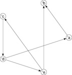
coords for every node, one can then define functions that mark the nodes with small disks and draws lines or arrows between the nodes to represent the edges. This is stuff that one would expect to find in some standard extension, but at the moment one is out of luck in this regard. Instead, a simple example with a very basic layout is provided here.
| Minimalistic graph layout |
|---|
 |
|
Placing the nodes on a circle and basic rendering of the nodes and edges. Note that two reciprocal directed edges will come out as one stroke with arrowheads in both ends.
|
|
| Source:
show/hide
—
visit
|
##needs ..Shapes..Data / seq-support

##lookin ..Shapes
##lookin ..Shapes..Data
##lookin ..Shapes..Geometry
##lookin ..Shapes..Layout
##lookin ..Shapes..Graphics

/** Graph layout function for nodes on a circle.
 ** (Ignoring any previous content of node values.)
 **/
circleGraphLayout: \ g radius:3cm →
{
  delta: 360° / g.node_count
  [g.with_node_values [fmap (\ node → (> coords:radius*[dir node.index*delta] <)) g.nodes]]
}

/** Basic rendering of a graph with nodes layout.
 **/
renderGraph: \ g →
{
  nodeRadius: 0.75*Text..@size

  /** A circle at each node **/
  nodeCircles: [g.nodes.foldl \ s n → (s & [[shift n.value.coords] stroke[][circle nodeRadius]]) null]

  /**  the node keys **/
  nodeKeys: [g.nodes.foldl \ s n → (s & [[shift n.value.coords] (Text..newText << (String..newString << n.key) ) >> center_x >> [shift (0,~0.5*nodeRadius)]]) null]

  /** Stroke the edges **/
  edgePath: \ e →
  {
    source: e.source.value.coords
    target: e.target.value.coords
    tmp: source--target
    (source + nodeRadius * tmp.begin.T)--(target + nodeRadius * tmp.end.rT)
  }
  edgeArrow: [ShapesArrow width:4bp ...]
  edgeStrokes: [g.edges.foldl \ s e → (s & [stroke [edgePath e] head:[if e.directed? edgeArrow NO_ARROW]]) null]

  nodeCircles & nodeKeys & edgeStrokes
}

/** Example graph.
 **/
g: [graph directed:true
     nodes: [list 'a 'b 'c 'd 'e]
     edges: [list (> 'a 'b <) (> 'c 'd <) (> 'd 'a <) (> 'd 'e <) (> 'e 'b <) (> 'e 'c <) ]
   ]

/** Apply layout and rendering functions.
 **/
Text..@size:9bp & Traits..@width:0.3bp | [renderGraph [circleGraphLayout g]]
|
A
bipartite graph is a graph where the nodes are divided into two partitions, and the two nodes incident to an edge are not allowed to belong to the same partition. The idea can be extended to any number of partitions, but two is by far the most common. The
§Graph type allows any number of partitions, but this guide will only consider the case of two groups, the generalization is trivial.
|
The definition used here for bipartite is not the only one with widespread use. It is also common to refer to a graph as bipartite if its nodes can be divided into two groups such that all edges go between the groups.
|
The partitions are identified by keys, similar to how nodes are identified, and the set of all possible keys has to be given explicitly. When a set of partition keys is present, the graph is partitioned by definition, and each node must be assigned one of these keys. For example, here is a bipartite graph with the partitions identified by the keys
'left and
'right (the node partition can be given as the third ordered member of the node data, after the node key and value):
[graph undirected:true partitions:[list 'left 'right]
  nodes: [list (> 'a 1 'left <) (> 'b 2 'left <) (> 'c 3 'left <)
               (> 'A 9 'right <) (> 'B 8 'right <) (> 'C 3 'right <)
         ]
  edges: [list (> 'a 'A <) (> 'a 'C <) (> 'b 'A <) (> 'c 'C <)]
]
| Bipartite graph |
|---|
 |
|
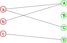
Illustration of a bipartite graph. Note that all edges connect two nodes of different color.
|
|
| Source:
show/hide
—
visit
|
##needs ..Shapes..Data / seq-support

##lookin ..Shapes
##lookin ..Shapes..Data
##lookin ..Shapes..Geometry
##lookin ..Shapes..Layout
##lookin ..Shapes..Graphics

/** Graph layout function for bipartite graphs.
 ** (Ignoring any previous content of node values.)
 **/
bipartiteGraphLayout: \ g partitionSep:5cm nodeSep:1cm →
{
  dx: partitionSep / 2
  leftKey: [seq_index '0 g.partitions]
  rightKey: [seq_index '1 g.partitions]
  leftYHigh: nodeSep * 0.5 * ([g.partition_node_count leftKey] - '1)
  rightYHigh: nodeSep * 0.5 * ([g.partition_node_count rightKey] - '1)
  nodeValues:
    seq_reverse [] [g.nodes.foldl
      ( \ p n →
        [if n.partition = leftKey
          (>
            res: (> coords: (~dx, leftYHigh - p.iLeft * nodeSep) <) ; p.res
            iLeft: p.iLeft + '1
            iRight: p.iRight
          <)
          (>
            res: (> coords: (dx, rightYHigh - p.iRight * nodeSep) <) ; p.res
            iLeft: p.iLeft
            iRight: p.iRight + '1
          <)
        ]
      )
      (> res:nil iLeft:'0 iRight:'0 <)
    ].res
  [g.with_node_values nodeValues]
}

/** Basic rendering of a graph with nodes layout.
 **/
renderBipartiteGraph: \ g →
{
  nodeRadius: 0.75*Text..@size
  leftKey: [seq_index '0 g.partitions]

  /** A circle at each node **/
  nodeCircles: Traits..@width:3*Traits..@width | [g.nodes.foldl \ s n → (s & ( Traits..@stroking:[if n.partition = leftKey Traits..RGB..RED Traits..RGB..GREEN] | [[shift n.value.coords] stroke[][circle nodeRadius]] ) ) null]

  /**  the node keys **/
  nodeKeys: [g.nodes.foldl \ s n → (s & [[shift n.value.coords] (Text..newText << (String..newString << n.key) ) >> center_x >> [shift (0,~0.5*nodeRadius)]]) null]

  /** Stroke the edges **/
  edgePath: \ e →
  {
    source: e.source.value.coords
    target: e.target.value.coords
    tmp: source--target
    (source + nodeRadius * tmp.begin.T)--(target + nodeRadius * tmp.end.rT)
  }
  edgeArrow: [ShapesArrow width:4bp ...]
  edgeStrokes: [g.edges.foldl \ s e → (s & [stroke [edgePath e] head:[if e.directed? edgeArrow NO_ARROW]]) null]

  nodeCircles & nodeKeys & edgeStrokes
}

/** Example graph.
 **/
g: [graph undirected:true partitions:[list 'left 'right]
      nodes: [list (> 'a 1 'left <) (> 'b 2 'left <) (> 'c 3 'left <)
                   (> 'A 9 'right <) (> 'B 8 'right <) (> 'C 3 'right <) (> 'D 1 'right <)
             ]
      edges: [list (> 'a 'A <) (> 'a 'C <) (> 'b 'A <) (> 'c 'D <)]
   ]

/** Apply layout and rendering functions.
 **/
Text..@size:9bp & Traits..@width:0.3bp | [renderBipartiteGraph [bipartiteGraphLayout g]]
|
A
multigraph is a graph where parallel edges are allowed. Since the two nodes incident to an edge cannot be used to uniquely identify an edge in a multigraph, each edge may additionally carry a label. The purpose of the label is only to make the edge uniquely identifiable; if you are considering using the label for something else, it is probably better to put that information in the edge value instead. Here is a simple example of a graph with parallel edges:
[graph undirected:true parallel:true
  nodes: [list 'a 'b 'c]
  edges: [list
           (> 'a 'b label:'even <) (> 'a 'b label:'odd <)
           (> 'a 'c label:'even <) (> 'a 'c label:'odd <)
           (> 'b 'c label:'even <) (> 'b 'c label:'odd <)
           (> 'c 'b label:'even <) (> 'c 'b label:'odd <)
         ]
]
As this example shows, there is no requirement that the edge labels be globally unique in the graph. On the contrary, it may be useful to group edges together by giving them the same key. It is even allowed to have parallel edges with the same key, although that defeats the purpose of being able to uniquely identify the edges.
As an alternative to working with all the individual edges of a multigraph, it is possible to work with
multiedges (of type
§MultiEdge) instead. A multiedge is a grouping of parallel edges, and can neither have an index, a label nor a value. In a limited way, it allowed the graph to be treated as if there were no parallel edges.
At the time of writing, multiedges are not stored in the §Graph values. Instead, they are constructed as needed, and if execution time is a priority, the user should take measures to reduce the number of times the multiedges get constructed. Getting the all multiedges in the graph takes time linear in the number of edges in the graph, but finding all multiedges incident to a node is not linear in the node's degree.
|
| Multigraph |
|---|
 |
|
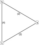
Illustration of a multigraph. Instead of showing the individual edges, multiedges are shown instead. The multiplicity of a multiedge is displayed by the edge.
|
|
| Source:
show/hide
—
visit
|
##needs ..Shapes..Data / seq-support

##lookin ..Shapes
##lookin ..Shapes..Data
##lookin ..Shapes..Geometry
##lookin ..Shapes..Layout
##lookin ..Shapes..Graphics

/** Graph layout function for nodes on a circle.
 ** (Ignoring any previous content of node values.)
 **/
circleGraphLayout: \ g radius:3cm →
{
  delta: 360° / g.node_count
  [g.with_node_values [fmap (\ node → (> coords:radius*[dir node.index*delta] <)) g.nodes]]
}

/** Basic rendering of a graph with nodes layout.
 **/
renderMultiGraph: \ g →
{
  /** Rendering parameters **/
  nodeRadius: 0.75 * Text..@size
  multiplicityRadius: 0.7 * Text..@size

  /** A circle at each node. **/
  nodeCircles: [g.nodes.foldl \ s n → (s & [[shift n.value.coords] stroke[][circle nodeRadius]]) null]

  /** Node keys. **/
  nodeKeys: [g.nodes.foldl \ s n → (s & [[shift n.value.coords] (Text..newText << (String..newString << n.key) ) >> center_x >> [shift (0,~0.5*nodeRadius)]]) null]

  /** Draw each multiedge as a straigt line between the nodes. **/
  edgePath: \ me →
  {
    source: me.source.value.coords
    target: me.target.value.coords
    tmp: source--target
    (source + nodeRadius * tmp.begin.T)--(target + nodeRadius * tmp.end.rT)
  }

  /** Arrow head for directed multiedges. **/
  edgeArrow: [ShapesArrow width:4bp ...]

  /** A label showing the multiplicity of a multiedge, positioned inside an imaginary circle of radius multiplicityRadius. **/
  multiplicityLabel: \ count →
    (Text..newText << (String..newString << [String..sprintf `(%d)´ count]) ) >> center_x >> [shift (0,~0.5 * multiplicityRadius)]

  /** Stroke an edge path and add a multiplicity label to the side of the stroke. **/
  drawMultiEdge: \ me →
  {
    p: [edgePath me]
    sl: [p [Numeric..Math..abs p]/2]
    (Traits..@width: 3 * Traits..@width | [stroke p head:[if me.directed? edgeArrow NO_ARROW]])
    &
    [[shift sl.p + sl.N * multiplicityRadius] [multiplicityLabel me.count]]
  }

  /** Draw all edges. **/
  edgeStrokes: [g.multiedges.foldl \ s me → (s & [drawMultiEdge me]) null]

  /** Combine all results. **/
  nodeCircles & nodeKeys & edgeStrokes
}

/** Example graph.
 **/
g: [graph undirected:true parallel:true
      nodes: [list 'a 'b 'c]
      edges: [list
               (> 'a 'b label:'even <) (> 'a 'b label:'odd <)
               (> 'a 'c label:'even <) (> 'a 'c label:'odd <)
               (> 'b 'c label:'even <) (> 'b 'c label:'odd <)
               (> 'c 'b label:'even <) (> 'c 'b label:'odd <)
             ]
   ]

/** Apply layout and rendering functions.
 **/
Text..@size:9bp & Traits..@width:0.3bp | [renderMultiGraph [circleGraphLayout g]]
|
A
mixed graph allows both directed and undirected edges. Here is a graph with both directed and undirected edges (with both types of edges allowed, each edge must specify its type):
[graph directed:true undirected:true
  nodes: [list 'a 'b 'c 'd]
  edges: [list
           (> 'a 'b directed:true <)
           (> 'b 'c directed:false <)
           (> 'c 'd directed:true <) (> 'd 'c directed:true <)
           (> 'd 'a directed:false <) (> 'd 'a directed:true <) (> 'a 'd directed:true <)
           (> 'a 'c directed:false <) (> 'a 'c directed:true <)
         ]
]
Sometimes, one can address problems in mixed graphs by replacing all undirected edges with a pair of reciprocal directed edges. In general, this leads to a directed graph with parallel edges, so then one has to tackle parallel edges instead of the mix of undirected and directed edges.
As an alternative to destroying the mixed structure of the graph, one can try to express algorithms without reference to whether edges are directed or undirected. For example, one can visit all the nodes along a
§Walk in a mixed graph by calling the
§Node method
trace on successive edges in the walk.
|
The example below needs a sorting function in order to group all edges incident to a pair of nodes. Doing this without sorting would be possible, but it would be a very inefficient solution.
|
| Mixed graph |
|---|
 |
|
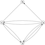
Illustration of a mixed graph. Unlike the basic rendering example above, we now take measures to avoid that edge strokes end up on top of each other.
|
|
| Source:
show/hide
—
visit
|
##needs ..Shapes..Data / seq-support

##lookin ..Shapes
##lookin ..Shapes..Data
##lookin ..Shapes..Geometry
##lookin ..Shapes..Layout
##lookin ..Shapes..Graphics

/** Graph layout function for nodes on a circle.
 ** (Ignoring any previous content of node values.)
 **/
circleGraphLayout: \ g radius:3cm →
{
  delta: 360° / g.node_count
  [g.with_node_values [fmap (\ node → (> coords:radius*[dir node.index*delta] <)) g.nodes]]
}

/** Group all edges incident to the same nodes (independenty of directedness and direction).
 **/
groupMixedEdges:
{
  /** Test if two edges are incident to the same vertices.
   **/
  sameIncidentVertices: \ e f →
  {
    e1: e.source.index
    e2: e.target.index
    f1: f.source.index
    f2: f.target.index
    [Numeric..Math..min e1 e2] = [Numeric..Math..min f1 f2] and [Numeric..Math..max e1 e2] = [Numeric..Math..max f1 f2]
  }

  /** Sort a group of edges such that parallel edges are adjacent in the sequence.
   **/
  sortEdgeGroup: \ edgesVec →
  {
    edges: edgesVec.list
    sortKeys: [fmap ( \ e → [array [if e.directed? [if e.source.index < e.target.index '~1 '1] '0]] ) edges]
    array [] <>[unlist [lexiographicSort sortKeys edges]]
  }

  \ edges →
  {
    sortKeys: [fmap ( \ e → [array [Numeric..Math..min e.source.index e.target.index] [Numeric..Math..max e.source.index e.target.index]]) edges]
    edgesSorted: [lexiographicSort sortKeys edges]
    [fmap sortEdgeGroup [equivalent_runs sameIncidentVertices edgesSorted]]
  }
}

/** Rendering of a graph with nodes layout.
 **/
renderMixedGraph: \ g →
{
  nodeRadius: 0.75*Text..@size

  /** A circle at each node **/
  nodeCircles: [g.nodes.foldl \ s n → (s & [[shift n.value.coords] stroke[][circle nodeRadius]]) null]

  /**  the node keys **/
  nodeKeys: [g.nodes.foldl \ s n → (s & [[shift n.value.coords] (Text..newText << (String..newString << n.key) ) >> center_x >> [shift (0,~0.5*nodeRadius)]]) null]

  /** Stroke the edges **/
  edgePath: \ e angleOffset →
  {
    rev: e.source.index > e.target.index
    (< v w >): [if rev (> e.target e.source <) (> e.source e.target <)]
    p1: v.value.coords
    p2: w.value.coords
    tmp: p1--p2
    a1: [angle tmp.begin.T] + angleOffset
    a2: [angle tmp.end.rT] - angleOffset
    pth: (p1 + nodeRadius * [dir a1])>(1%C ^ a1)--(1%C ^ a2)<(p2 + nodeRadius * [dir a2])
    [if rev [reverse pth] pth]
  }
  edgeArrow: [ShapesArrow width:4bp ...]

  drawEdgeGroup: \ edges →
  {
    n: edges.size
    angleMax: [Numeric..Math..arctan 0.577350269 * (n - '1)] / 3
    [if n = '1
      {
        e: [edges '0]
        [stroke [edgePath e 0.0] head:[if e.directed? edgeArrow NO_ARROW]]
      }
      [edges.range.foldl
        \ s i →
        {
          e: [edges i]
          s
          &
          [stroke
            [edgePath e angleMax * ( (2 * i) / (n - '1) - 1 )]
            head:[if e.directed? edgeArrow NO_ARROW]
          ]
        }
        null
      ]
    ]
  }

  edgeStrokes:
    [[groupMixedEdges g.edges].foldl
       \ s edgeGroup → (s & [drawEdgeGroup edgeGroup])
       null
    ]

  nodeCircles & nodeKeys & edgeStrokes
}

/** Example graph.
 **/
g: [graph directed:true undirected:true
     nodes: [list 'a 'b 'c 'd]
     edges: [list
              (> 'a 'b directed:true <)
              (> 'b 'c directed:false <)
              (> 'c 'd directed:true <) (> 'd 'c directed:true <)
              (> 'd 'a directed:false <) (> 'd 'a directed:true <) (> 'a 'd directed:true <)
              (> 'a 'c directed:false <) (> 'a 'c directed:true <)
            ]
   ]

/** Apply layout and rendering functions.
 **/
Text..@size:9bp & Traits..@width:0.3bp | [renderMixedGraph [circleGraphLayout g]]
|
Below are some ideas for future developments related to graphs.
- Finalizing the design for hierarchical graphs, and implement it.
- Adding functions for importing and exporting graph data in the GEFX format (there are many other formats out there as well, but this one seems to have outstanding documentation as well as good tool support).
- A standard Shapes extension for graph layout.
